Calculate Technical Analysis Indicators with Pandas

header-1

In finance, technical analysis is an analysis methodology for forecasting the direction of prices through the study of past market data, primarily price and volume. Technical analysts rely on a combination of technical indicators to study a stock and give insight about trading strategy. Common technical indicators like SMA and Bollinger Band® are widely used. Here is a list of technical indicators.

In a previous story, I talked about how to collect such information with Pandas. In this story, I will demonstrate how to compute Bollinger Bands® and use it to provide potential buy / sell signals.

Bollinger Bands®

Bollinger Bands is used to define the prevailing high and low prices in a market to characterize the trading band of a financial instrument or commodity. Bollinger Bands are a volatility indicator. Bands are consists of Moving Average (MA) line, a upper band and lower band. The upper and lower bands are simply MA adding and subtracting standard deviation. Standard deviation is a measurement of volatility. That’s why it’s a volatility indictor.

Upper Band = (MA + Kσ)
Lower Band = (MA − Kσ)

MA is typical 20 day moving average and K is 2. I will use them in this example.

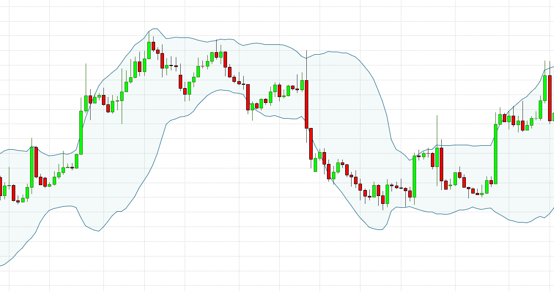example of Bollinger Bands Prerequisite environment setup (follow Step1 in this post)

Data:

We will use a csv file (AMZN.csv) collected from the previous post in this example

Code:

import pandas as pd
import matplotlib.pyplot as plt

symbol='AMZN'
# read csv file, use date as index and read close as a column
df = pd.read_csv('~/workspace/{}.csv'.format(symbol), index_col='date',
                 parse_dates=True, usecols=['date', 'close'],
                 na_values='nan')
# rename the column header with symbol name
df = df.rename(columns={'close': symbol})
df.dropna(inplace=True)

# calculate Simple Moving Average with 20 days window
sma = df.rolling(window=20).mean()

# calculate the standar deviation
rstd = df.rolling(window=20).std()

upper_band = sma + 2 * rstd
upper_band = upper_band.rename(columns={symbol: 'upper'})
lower_band = sma - 2 * rstd
lower_band = lower_band.rename(columns={symbol: 'lower'})

df = df.join(upper_band).join(lower_band)
ax = df.plot(title='{} Price and BB'.format(symbol))
ax.fill_between(df.index, lower_band['lower'], upper_band['upper'], color='#ADCCFF', alpha='0.4')
ax.set_xlabel('date')
ax.set_ylabel('SMA and BB')
ax.grid()
plt.show()

Output

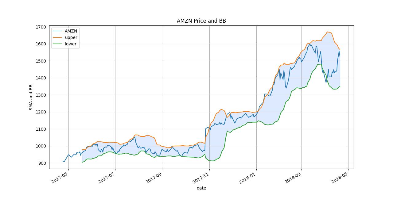
Amazon price and its Bollinger Bands Interpretation of Buy / Sell signals

Approximately 90% of price action between the two bands. Therefore the bands can be used to identify potential overbought or oversold conditions. If stock price breaks out the upper band, it could be an overbought condition (indication of short). Similarly, when it breaks out the lower band, it could be oversold condition (indication of long). But Bollinger Bands is not a standalone system that always gives accurate buy / sell signals. One should consider the overall trend with the bands to identify the signal. Otherwise, with only Bollinger Bands, one could make wrong orders constantly. In the above Amazon example, the trend is up. So one should only take long positions when the lower band is tagged. More information could be found here.

That’s how easy to compute technical indicators with 🐼!

I have written a post about how to use TA to compute the indicators.