
How to use TA-Lib for Technical Analysis in Python

In finance, a trading strategy is a fixed plan that is designed to achieve a profitable return by going long or short in markets. The main reasons that a properly researched trading strategy helps are its verifiability, quantifiability, consistency, and objectivity. For every trading strategy one needs to define assets to trade, entry/exit points and money management rules. Bad money management can make a potentially profitable strategy unprofitable. — From Wikipedia
Strategies are categorized as fundamental analysis based and technical analysis based. While fundamental analysis focus on company’s assets, earnings, market, dividend etc, technical analysis solely focus on its stock price and volume. Technical analysis widely use technical indicators which are computed with price and volume to provide insights of trading action. Technical indicators further categorized in volatility, momentum, trend, volume etc. Selectively combining indicators for a stock may yield great profitable strategy. Once a strategy is built, one should backtest the strategy with simulator to measure performance (return and risk) before live trading. I have another post covering backtest with backtrader.
As technical indicators play important roles in building a strategy, I will demonstrate how to use TA-Lib to compute technical indicators and build a simple strategy. (Please do not directly use the strategy for live trading as backtest is required). If you want to calculate the indicator by yourself, refer to my previous post on how to do it in Pandas.
In this post, I will build a strategy with RSI (a momentum indicator) and Bollinger Bands %b (a volatility indicator). High RSI (usually above 70) may indicate a stock is overbought, therefore it is a sell signal. Low RSI (usually below 30) indicates stock is oversold, which means a buy signal. Bollinger Bands tell us most of price action between the two bands. Therefore, if %b is above 1, price will likely go down back within the bands. Hence, it is a sell signal. While if it is lower than 0, it is considered a buy signal. The strategy is a simple voting mechanism. When two indicators think it is time to buy, then it issues buy order to enter. When both indicators think it is time to sell, then it issues sell order to exit.
To install TA-Lib and other dependencies on Mac
python3 -m venv tutorial-env
source ~/tutorial-env/bin/activate
pip install panda
pip install pandas_datareader
pip install matplotlib
pip install scipy
pip install cython
brew install ta-lib
pip install TA-lib
Compute Bollinger Bands or RSI
import pandas_datareader.data as web
import pandas as pd
import numpy as np
from talib import RSI, BBANDS
import matplotlib.pyplot as plt
start = '2015-04-22'
end = '2017-04-22'

symbol = 'MCD'
max_holding = 100
price = web.DataReader(name=symbol, data_source='quandl', start=start, end=end)
price = price.iloc[::-1]
price = price.dropna()
close = price['AdjClose'].values
up, mid, low = BBANDS(close, timeperiod=20, nbdevup=2, nbdevdn=2, matype=0)
rsi = RSI(close, timeperiod=14)
print("RSI (first 10 elements)\n", rsi[14:24])
Output
RSI (first 10 elements)
 [50.45417011 47.89845022 49.54971141 51.0802541  50.97931103 61.79355957
 58.80010324 54.64867736 53.23445848 50.65447261]
Convert Bollinger Bands to %b
def bbp(price):
    up, mid, low = BBANDS(close, timeperiod=20, nbdevup=2, nbdevdn=2, matype=0)
    bbp = (price['AdjClose'] - low) / (up - low)
    return bbp
Compute the holdings based on the indicators
holdings = pd.DataFrame(index=price.index, data={'Holdings': np.array([np.nan] * index.shape[0])})
holdings.loc[((price['RSI'] < 30) & (price['BBP'] < 0)), 'Holdings'] = max_holding
holdings.loc[((price['RSI'] > 70) & (price['BBP'] > 1)), 'Holdings'] = 0
holdings.ffill(inplace=True)
holdings.fillna(0, inplace=True)
Further, we should get the trading action based on the holdings

holdings['Order'] = holdings.diff()
holdings.dropna(inplace=True)
Let’s visualize our action and indicators
fig, (ax0, ax1, ax2) = plt.subplots(3, 1, sharex=True, figsize=(12, 8))
ax0.plot(index, price['AdjClose'], label='AdjClose')
ax0.set_xlabel('Date')
ax0.set_ylabel('AdjClose')
ax0.grid()
for day, holding in holdings.iterrows():
    order = holding['Order']
    if order > 0:
        ax0.scatter(x=day, y=price.loc[day, 'AdjClose'], color='green')
    elif order < 0:
        ax0.scatter(x=day, y=price.loc[day, 'AdjClose'], color='red')

ax1.plot(index, price['RSI'], label='RSI')
ax1.fill_between(index, y1=30, y2=70, color='#adccff', alpha='0.3')
ax1.set_xlabel('Date')
ax1.set_ylabel('RSI')
ax1.grid()

ax2.plot(index, price['BB_up'], label='BB_up')
ax2.plot(index, price['AdjClose'], label='AdjClose')
ax2.plot(index, price['BB_low'], label='BB_low')
ax2.fill_between(index, y1=price['BB_low'], y2=price['BB_up'], color='#adccff', alpha='0.3')
ax2.set_xlabel('Date')
ax2.set_ylabel('Bollinger Bands')
ax2.grid()

fig.tight_layout()
plt.show()
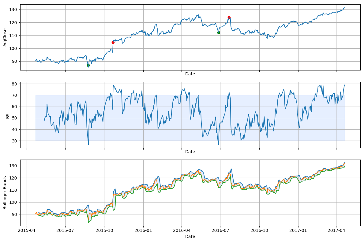
The below, I plot the action with green points (entry points) and red points (exit points) with the Adjusted Close Price of the McDonald (2015 April to 2017 April). Alongside, the RSI indicators and Bollinger Bands are plotted to show how two indicators contribute to a trading action. From the graph, it shows the strategy is good. It captures a couple relative some low prices and high price during the period. One should backtest to get how well the strategy does compared to benchmark.
Result in graph
If you would like to learn more about Machine Learning there is a helpful series of courses in educative.io. These courses cover topics like basic ML, NLP, Image Recognition etc.