
Get Trading Data with Pandas Library

Pandas is an open source, library providing high-performance, easy-to-use data structures and data analysis tools for the Python programming language. Pandas is one of the most popular tools for trading strategy development, because Pandas has a wide variety of utilities for data collection, manipulation and analysis, etc.
For quantitative analysts who believe in trading, they need access to stock price and volume so that they can compute a combination of technical indicators (e.g. SMA, BBP, MACD etc.) for strategy. Luckily, such data is available on many platforms (e.g. IEX, Quandl) via REST APIs. Even more luckily, pandas_datareader provides a consistent simple API for you to collect data from these platforms. In this story, I will walk through how to collect stock data with Pandas.
Prerequisite: Python 3
Step1: Environment setup (virtual env)
python3 -m venv tutorial-env
source ~/tutorial-env/bin/activate
pip install panda
pip install pandas_datareader
pip install matplotlib
pip install scipy
(Don’t forget to activate the environment source ~/tutorial-env/bin/activate or choose the virtual env in your IDE)
Step2: Code (fetching data and dump to a csv file)
import matplotlib.pyplot as plt
import pandas_datareader.data as web
# collect data for Amazon from 2017-04-22 to 2018-04-22
start = '2017-04-22'
end = '2018-04-22'
df = web.DataReader(name='AMZN', data_source='iex', start=start, end=end)
print(df)
df.to_csv("~/workspace/{}.csv".format(symbol))
Output of Dataframe
open       high        low    close    volume
date
2017-04-24   908.680   909.9900   903.8200   907.41   3122893
2017-04-25   907.040   909.4800   903.0000   907.62   3380639
2017-04-26   910.300   915.7490   907.5600   909.29   2608948
2017-04-27   914.390   921.8600   912.1100   918.38   5305543
2017-04-28   948.830   949.5900   924.3335   924.99   7364681
2017-05-01   927.800   954.4000   927.8000   948.23   5466544
2017-05-02   946.645   950.1000   941.4130   946.94   3848835
2017-05-03   946.000   946.0000   935.9000   941.03   3582686
2017-05-04   944.750   945.0000   934.2150   937.53   2418381
...
A corresponding csv file is saved in an ouput directory (~/workspace/AMZN.csv) in this example.
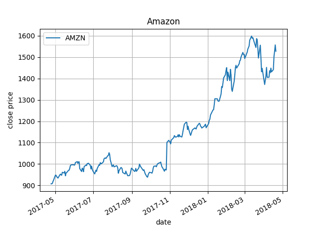
Step3: Visualize what was collected with matplotlib
# select only close column
close = df[['close']]
# rename the column with symbole name
close = close.rename(columns={'close': symbol})
ax = close.plot(title='Amazon')
ax.set_xlabel('date')
ax.set_ylabel('close price')
ax.grid()
plt.show()
That’s it! Now you have downloaded stock data for analysis.
The whole example
import pandas_datareader.data as web
import matplotlib.pyplot as plt

# collect data for Amazon from 2017-04-22 to 2018-04-22
start = '2017-04-22'
end = '2018-04-22'
symbol='AMZN'
df = web.DataReader(name=symbol, data_source='iex', start=start, end=end)
df.index = df.index.to_datetime()
print(df)
df.to_csv("~/workspace/{}.csv".format(symbol))
# select only close column
close = df[['close']]
# rename the column with symbole name
close = close.rename(columns={'close': symbol})
ax = close.plot(title='Amazon')
ax.set_xlabel('date')
ax.set_ylabel('close price')
ax.grid()
plt.show()
More data analysis with Pandas can be found here!
Last words, if you feel more comfortable with Excel and interested to analyze stocks easily, Guang Mo has a post about collecting data with Intrinio Excel addin.