
Portfolio Optimization for Minimum Risk with Scipy — Efficient Frontier Explained with SciPy

Beyond the bound
Given 4 assets’ risk and return as following, what could be the risk-return for any portfolio built with the assets. One may think that all possible values have to fall inside the convex hull. But it is possible to go beyond the bond, if you consider the correlation coefficient among the assets. That’s being said combining inversely correlated assets can construct a portfolio with lower risk. More details can be found in my previous post.
To demonstrate portfolio risk-return can go beyond the area, I get 3000 samples of randomly-weighted portfolio and plot their risk-return.
Environment setup
Follow step 1 in this post
Compute and visualize assets return and risk
This is tutorial, we pick 4 stocks BA (Boeing), C (Citigroup), AAL (American Airlines Group), NFLX (Netflix) from 4 different sectors for analysis. As my previous post, risk is measured by daily return’s standard deviation. The return is computed as below
K * (expected return – expected risk free rate)
K is the square root of frequency of sampling. That means if we measure with daily return, K is sqrt(250) (There are roughly 250 trading days in a year). Treasury rate is commonly used as risk free rate. In this tutorial, we will use 0.
Code
scatter plotting the individual asset risk-return
import pandas_datareader.data as web
import pandas as pd
import matplotlib.pyplot as plt
import numpy as np
from scipy.optimize import minimize
def get_risk(prices):
    return (prices / prices.shift(1) - 1).dropna().std().values

def get_return(prices):
    return ((prices / prices.shift(1) - 1).dropna().mean() * np.sqrt(250)).values
symbols = ['BA', 'C', 'AAL', 'NFLX']
prices = pd.DataFrame(index=pd.date_range(start, end))
for symbol in symbols:
    portfolio = web.DataReader(name=symbol, data_source='quandl', start=start, end=end)
    close = portfolio[['AdjClose']]
    close = close.rename(columns={'AdjClose': symbol})
    prices = prices.join(close)
    portfolio.to_csv("~/workspace/{}.csv".format(symbol))
prices = prices.dropna()
risk_v = get_risk(prices)
return_v = get_return(prices)
fig, ax = plt.subplots()
ax.scatter(x=risk_v, y=return_v, alpha=0.5)
ax.set(title='Return and Risk', xlabel='Risk', ylabel='Return')
for i, symbol in enumerate(symbols):
    ax.annotate(symbol, (risk_v[i], return_v[i]))
plt.show()
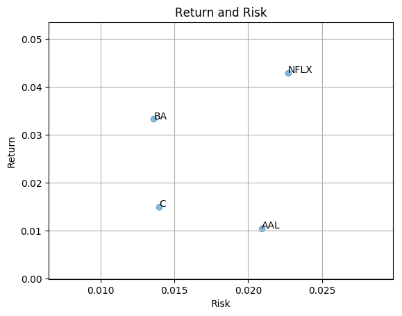
Return and risk for BA (Boeing), C (Citigroup), AAL (American Airlines Group), NFLX (Netflix)
Build portfolio with random weights
def random_weights(n):
    weights = np.random.rand(n)
    return weights / sum(weights)
def get_portfolio_risk(weights, normalized_prices):
    portfolio_val = (normalized_prices * weights).sum(axis=1)
    portfolio = pd.DataFrame(index=normalized_prices.index, data={'portfolio': portfolio_val})
    return (portfolio / portfolio.shift(1) - 1).dropna().std().values[0]
def get_portfolio_return(weights, normalized_prices):
    portfolio_val = (normalized_prices * weights).sum(axis=1)
    portfolio = pd.DataFrame(index=normalized_prices.index, data={'portfolio': portfolio_val})
    ret = get_return(portfolio)
    return ret[0]
risk_all = np.array([])
return_all = np.array([])
# for demo purpose, plot 3000 random portoflio
np.random.seed(0)
normalized_prices = prices / prices.ix[0, :]
for _ in range(0, 3000):
    weights = random_weights(len(symbols))
    portfolio_val = (normalized_prices * weights).sum(axis=1)
    portfolio = pd.DataFrame(index=prices.index, data={'portfolio': portfolio_val})
    risk = get_risk(portfolio)
    ret = get_return(portfolio)
    risk_all = np.append(risk_all, risk)
    return_all = np.append(return_all, ret)
    p = get_portfolio_risk(weights=weights, normalized_prices=normalized_prices)
fig, ax = plt.subplots()
ax.scatter(x=risk_all, y=return_all, alpha=0.5)
ax.set(title='Return and Risk', xlabel='Risk', ylabel='Return')
for i, symbol in enumerate(symbols):
    ax.annotate(symbol, (risk_v[i], return_v[i]))
ax.scatter(x=risk_v, y=return_v, alpha=0.5, color='red')
ax.set(title='Return and Risk', xlabel='Risk', ylabel='Return')
ax.grid()
plt.show()
Risk comes from not knowing what you are doing — Warren Buffett
Let’s look at the risk and return. we do see that there are blue dots outside of the area. So diversification does help reduce the risk. But how do we find the best or efficient weight?
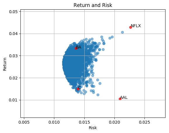
Return and risk of a portfolio of random weighted BA (Boeing), C (Citigroup), AAL (American Airlines Group), NFLX (Netflix) (3000 samples)
Efficient Frontier
From wikipedia, in modern portfolio theory, the efficient frontier (or portfolio frontier) is an investment portfolio which occupies the ‘efficient’ parts of the risk-return spectrum.
Here we will use scipy’s optimizer to get optimal weights for different targeted return. Note that, we have bounds that make sure weight are in range [0, 1] and constraints to ensure sum of weights is 1, also portfolio return meets our target return. With all this condition, scipy optimizer is able to find the best allocation.
# optimizer
def optimize(prices, symbols, target_return=0.1):
    normalized_prices = prices / prices.ix[0, :]
    init_guess = np.ones(len(symbols)) * (1.0 / len(symbols))
    bounds = ((0.0, 1.0),) * len(symbols)
    weights = minimize(get_portfolio_risk, init_guess,
                       args=(normalized_prices,), method='SLSQP',
                       options={'disp': False},
                       constraints=({'type': 'eq', 'fun': lambda inputs: 1.0 - np.sum(inputs)},
                                    {'type': 'eq', 'args': (normalized_prices,),
                                     'fun': lambda inputs, normalized_prices:
                                     target_return - get_portfolio_return(weights=inputs,
                                                                          normalized_prices=normalized_prices)}),
                       bounds=bounds)
    return weights.x
optimal_risk_all = np.array([])
optimal_return_all = np.array([])
for target_return in np.arange(0.005, .0402, .0005):
    opt_w = optimize(prices=prices, symbols=symbols, target_return=target_return)
    optimal_risk_all = np.append(optimal_risk_all, get_portfolio_risk(opt_w, normalized_prices))
    optimal_return_all = np.append(optimal_return_all, get_portfolio_return(opt_w, normalized_prices))
# plotting
fig, ax = plt.subplots()
# random portfolio risk return
ax.scatter(x=risk_all, y=return_all, alpha=0.5)
# optimal portfolio risk return
for i, symbol in enumerate(symbols):
    ax.annotate(symbol, (risk_v[i], return_v[i]))
ax.plot(optimal_risk_all, optimal_return_all, '-', color='green')
# symbol risk return
for i, symbol in enumerate(symbols):
    ax.annotate(symbol, (risk_v[i], return_v[i]))
ax.scatter(x=risk_v, y=return_v, color='red')
ax.set(title='Efficient Frontier', xlabel='Risk', ylabel='Return')
ax.grid()
plt.savefig('return_risk_efficient_frontier.png', bbox_inches='tight')
The green line indicate the efficient frontier. Now we know the best allocation with a given target return. Next question, what is the best allocation overall? Portfolio performance can be evaluated with return/risk ratio (known as Sharpe Ratio). High Sharpe Ratio indicates good balance of return and risk. This allocation can be found by drawing a Capital Allocation line that tangent to the efficient frontier. The tangent point is the allocation yields highest Sharpe ratio. To learn more, you can take a look at this article on how to find the highest sharpe ratio from the efficient frontier with Capital Allocation Line (CAL).

Efficient frontier — Return and risk of optimal asset-weights at different targeted returns That’s it. Now we know the theory of diversification. Happy investment and coding!